NFL Running Backs Interactive Visualization
Code for this project can be found at this repository
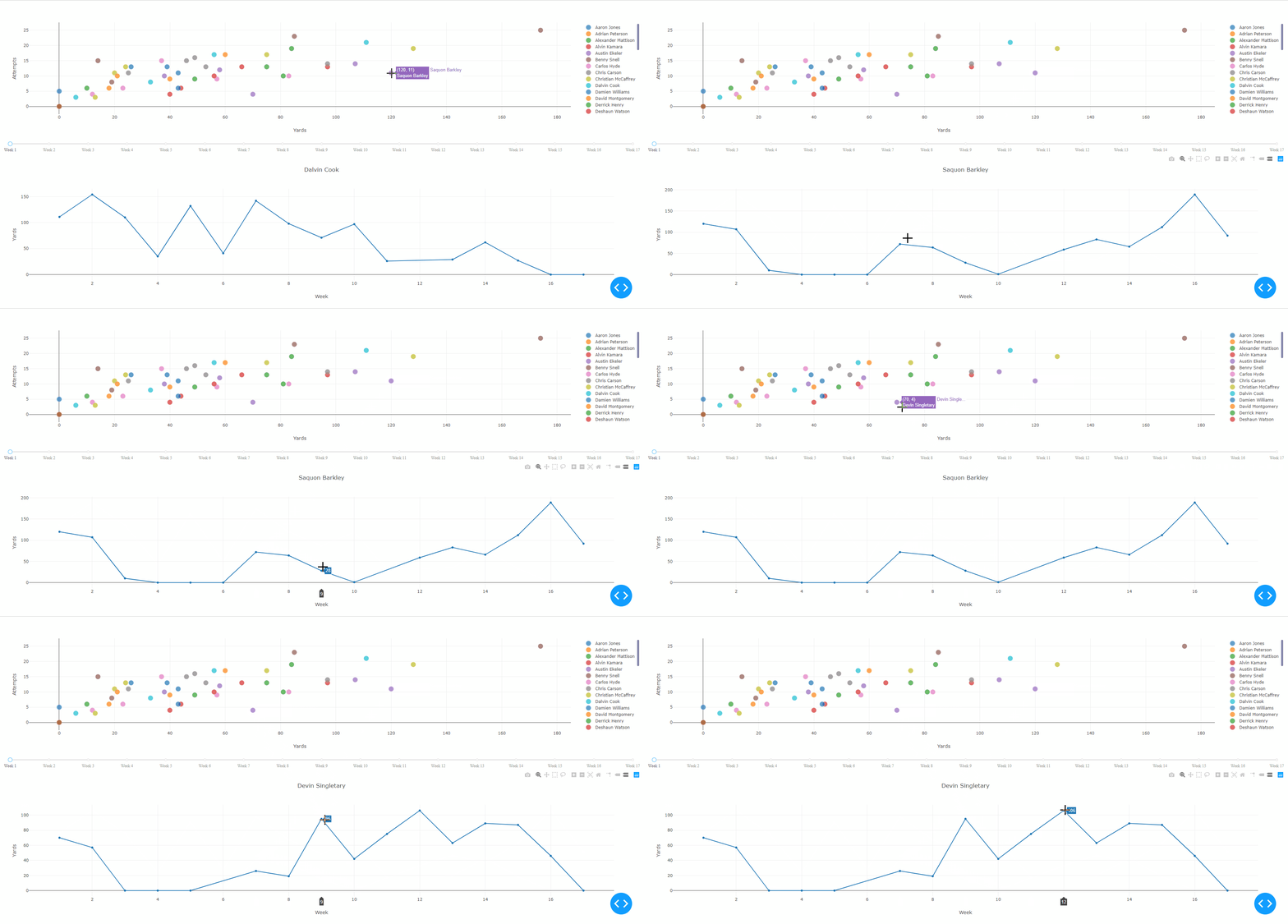
Interactive features include displaying player name with their respective yards and attempts on hover, as well as, a slider tool to change the week.

Clicking on a player’s point will display their weekly rushing performances over the entire season. Weeks without a point represent a bye for that player whereas a point with 0 indicates the player did not gain any yards due to injury, poor performance, being benched, et cetera.

Data Collection and Cleaning
To collect the data used for this project, I used the python libraries Requests and BeautifulSoup to scrape player statistics from NFL.com.
Requests allows python to easily make http requests and BeautifulSoup allows you to parse through and extract data from HTML an XML files.
Before scraping any website, you want to make sure you’re not attempting to extract any information the website owners wouldn’t want you to. To see what you’re allowed and not allowed to scrape through you can simply use the url’s /robots.txt.

Since the Disallow: does not include /player , the extension I used for player statistics, I am ok to scrape through without worrying about getting in trouble with NFL.com
The function I wrote to scrape each player’s gamelogs utilizes the libraries requests and BeautifulSoup which is aliased as soup.
def acquire_stats(url):
    r = requests.get(url)
    c = r.content

    page = soup(c,'html.parser')

    #data-table1 is the standard class for NFL.com stats tables
    reg = page.findAll("table",{"class":"data-table1"})
    for element in reg:
        if reg.index(element) == 1:
            table = element.find("tbody").findAll("tr") #for multiple tables in game logs, index 1 gives regular season
        elif len(reg) < 2:
            table = element.find("tbody").findAll("tr") #some pages only have regular season table


    #empty lists to append values to
    rows = []
    log = []

    #create a list with all of the td elements in the table
    for row in table:
        rows.append(row.findAll("td"))
    #iterate through the lists and retrieve the text elements, also removing line spacing characters
    for i in range(0,len(rows)):
        log.append([td.text.replace('\n','').replace('\t','').replace('\r','').replace('\xa0','').replace('@','') for td in rows[i]])
    del log[1::2]
    del reg
    del table
    return log
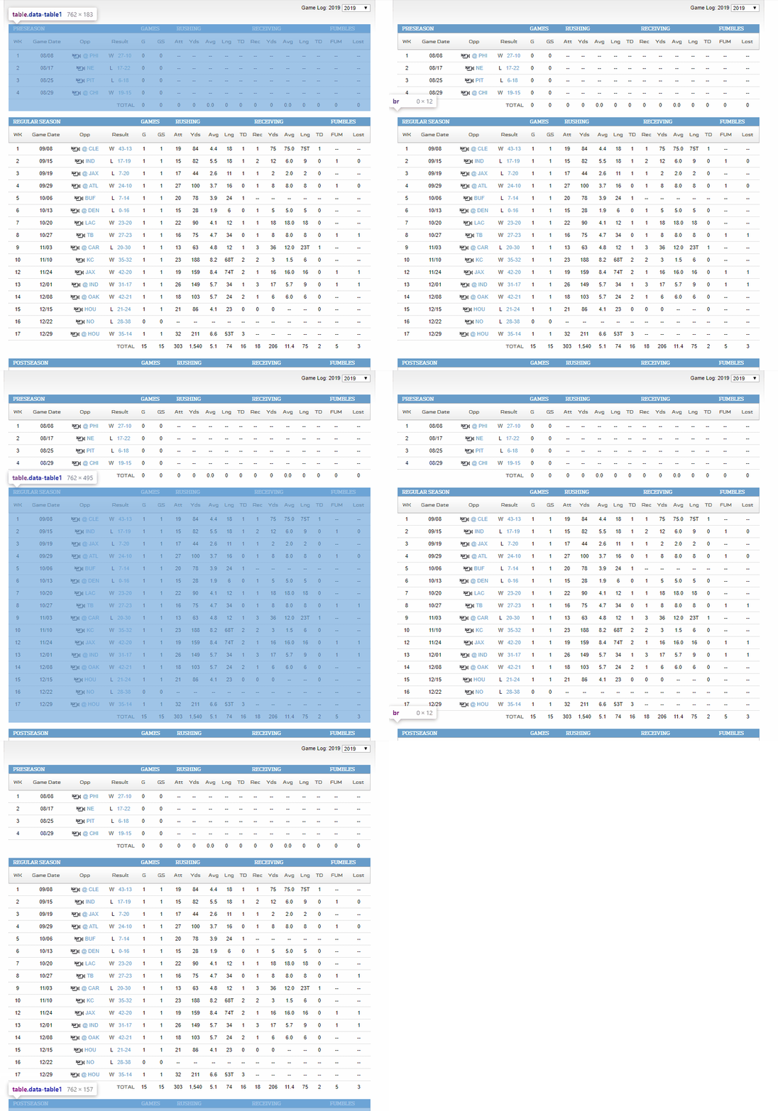
The function first passes in a url and uses requests to get the content of the specified url. BeautifulSoup is used to create a “soup” object from the HTML content which can then be easily parsed. Next, the function looks for all table elements which have the class "data-table1" since this is the uniform class given to all of NFL.com’s tables as seen below.

Since findAll creates a list of all of the elements it finds and I was only interested in looking at regular season statistics, the function assigns a value from the second element of the list. However, I found out that some player’s gamelogs only have a regular season table so the elif statement accounts for those players as well. The function then grabs all of the table rows and assigns it to a variable.
Finally the function iterates over the table rows, finding and cleaning all of the row elements, and appending all of the row elements to a list for the function to return.
I then created a list of urls from the top 50 rushers and used list comprehension, as well as the dict function, to create a dictionary where the keys are the player names and the values are nested lists containing the player’s weekly statistics.
Below is the first two weeks of Derrick Henry’s stats to show what the dict looks like
{'Derrick Henry': [['1','09/08','  CLE','W    43-13 ','1','1','19','84','4.4','18','1','1','75','75.0','75T','1','--','--'],
['2','09/15','  IND','L   17-19 ','1','1','15','82','5.5','18','1','2','12','6.0','9','0','1','0'],
Afterwards, I converted the dict of nested to lists into a dict of pandas dataframes where each key is the player’s name and the respective value is a dataframe corresponding to their regular season statistics, and an example can be seen below. I did this to simplify the process of giving the same column names for each player’s dataframe.
{'Derrick Henry':      0      1      2            3    4      5    6    7    8    9   10    11  \
 0    1  09/08    CLE  W    43-13     1      1   19   84  4.4   18    1     1
 1    2  09/15    IND   L   17-19     1      1   15   82  5.5   18    1     2
 2    3  09/19    JAX    L   7-20     1      1   17   44  2.6   11    1     1
 3    4  09/29    ATL  W    24-10     1      1   27  100  3.7   16    0     1
 4    5  10/06    BUF    L   7-14     1      1   20   78  3.9   24    1    --
 5    6  10/13    DEN    L   0-16     1      1   15   28  1.9    6    0     1
 6    7  10/20    LAC  W    23-20     1      1   22   90  4.1   12    1     1
 7    8  10/27     TB  W    27-23     1      1   16   75  4.7   34    0     1
 8    9  11/03    CAR   L   20-30     1      1   13   63  4.8   12    1     3
 9   10  11/10     KC  W    35-32     1      1   23  188  8.2  68T    2     2
 10  12  11/24    JAX  W    42-20     1      1   19  159  8.4  74T    2     1
 11  13  12/01    IND  W    31-17     1      1   26  149  5.7   34    1     3
 12  14  12/08    OAK  W    42-21     1      1   18  103  5.7   24    2     1
 13  15  12/15    HOU   L   21-24     1      1   21   86  4.1   23    0     0
 14  16  12/22     NO   L   28-38     0      0   --   --   --   --   --    --
 15  17  12/29    HOU  W    35-14     1      1   32  211  6.6  53T    3    --
 16      TOTAL     15           15  303  1,540  5.1   74   16   18  206  11.4

     12    13   14  15    16    17
 0   75  75.0  75T   1    --    --
 1   12   6.0    9   0     1     0
 2    2   2.0    2   0    --    --
 3    8   8.0    8   0     1     0
 4   --    --   --  --    --    --
 5    5   5.0    5   0    --    --
 6   18  18.0   18   0    --    --
 7    8   8.0    8   0     1     1
 8   36  12.0  23T   1    --    --
 9    3   1.5    6   0    --    --
 10  16  16.0   16   0     1     1
 11  17   5.7    9   0     1     1
 12   6   6.0    6   0    --    --
 13   0    --   --   0    --    --
 14  --    --   --  --    --    --
 15  --    --   --  --    --    --
 16  75     2    5   3  None  None  ,
Next I got rid of all of the columns which were not related to rushing statistics since that data would not be necessary for me to keep. In addition, I had to account for a few of the quarterbacks who were among the top 50 rushers since they had additional columns for passing statistics.
qbs = ['Lamar Jackson','Kyler Murray','Josh Allen','Deshaun Watson']
for player in stats:
    if player in qbs:
        #drops all columns not related to rushing for quarterbacks
        stats[player] = stats[player].drop(axis=1,labels=[6,7,8,9,10,11,12,13,14,15])
    elif player not in qbs:
        #drops all columns not related to rushing for runningbacks
        stats[player] = stats[player].drop(axis=1,labels=[11,12,13,14,15,16])
After some more cleaning, each player’s dataframe was reduced to contain only columns related to the week played, their opponent, and the rushing statistics for that week.
{'Derrick Henry':     week    opp   att    yds
                 0      1    CLE  19.0   84.0
                 1      2    IND  15.0   82.0
                 2      3    JAX  17.0   44.0
                 3      4    ATL  27.0  100.0
                 4      5    BUF  20.0   78.0
                 5      6    DEN  15.0   28.0
                 6      7    LAC  22.0   90.0
                 7      8     TB  16.0   75.0
                 8      9    CAR  13.0   63.0
                 9     10     KC  23.0  188.0
                 10    12    JAX  19.0  159.0
                 11    13    IND  26.0  149.0
                 12    14    OAK  18.0  103.0
                 13    15    HOU  21.0   86.0
                 14    16     NO   0.0    0.0
                 15    17    HOU  32.0  211.0,
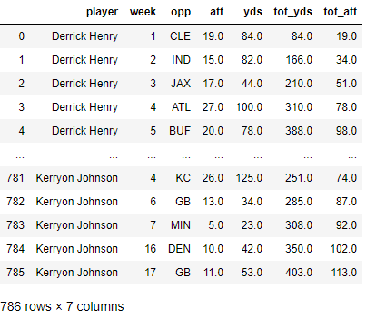
Then I created some additional columns containing the player’s name for each week they played, as well as, total yards and attempts at that point in the season. Finally, created a single dataframe from the dictionary values and exported the dataframe to csv.

Creating The Dash App
The final interactive visualization was created using Plotly’s library Dash which allows for easy creation of interactive analytics applications.
I started with importing the dash libraries I would be using along with pandas to read in the csv file.
import dash
import dash_core_components as dcc
import dash_html_components as html
from dash.dependencies import Input, Output
import pandas as pd
Next was reading in the csv and setting up the layout for the application.
df = pd.read_csv('https://raw.githubusercontent.com/a-camarillo/NFL-running-backs-2019/master/Data%20Cleaning/rushing_stats_2019')

app = dash.Dash(__name__)

app.layout = html.Div([
    html.Div([
        dcc.Graph(
            id='graph-with-slider',
            clickData={'points':[{'text': 'Dalvin Cook'}]}),
        dcc.Slider(
         id='week-slider',
         min=df['week'].min(),
         max=df['week'].max(),
         value=df['week'].min(),
         marks={str(week): 'Week {}'.format(week) for week in df['week'].unique()},
            step=None
        )
    ]),
    html.Div([
        dcc.Graph(id='line-graph')
    ])
])
The layout consists of two separate div elements which are wrapped inside a larger div element. The first element contains a graph,id='graph-with-slider', which uses clickData from a users click and a slider which contains a point for each unique value in the ‘week’ column of the dataframe. The second element contains the graph with id='line-graph'.
Finally, the functionality for the visualization which comes from utilizing Dash’s callback feature. Each callback has its own output, input, and function to be used by the callback.
@app.callback(
    Output('graph-with-slider', 'figure'),
    [Input('week-slider', 'value')])
def update_figure(selected_week):
    filtered_df = df[df.week == selected_week]
    traces = []
    for i in filtered_df.player.unique():
        df_by_player = filtered_df[filtered_df['player'] == i]
        traces.append(dict(
            x=df_by_player['tot_yds'],
            y=df_by_player['tot_att'],
            text=df_by_player['player'],
            mode='markers',
            opacity=0.7,
            marker={
                'size': 15,
                'line' : {'width': 0.5, 'color': 'white'}
            },
            name=i
        ))
    return {
        'data': traces,
        'layout':dict(
            xaxis={'type':'scatter','title':'Yards'},
            yaxis={'type':'scatter','title':'Attempts'},
            hovermode='closest',
            transition = {'duration': 500}
        )
    }
The first callback’s output is an updated figure for the graph-with-slider component and the input is the value of the slider. The update_figure function passes the value selected_week which is simply the input from the slider.
The function then creates a dataframe where the value for the week column is equal to the input value, iterates through the players creating a dictionary of the player and their stats for the respective week, and appends all of the dictionaries to an empty list.
The function returns two features for the output figure graph-with-slider: the data for the figure which is the final list of player dicts and the layout which creates the scatter points and annotations. The output now updates whenever a new input(slider value) is passed.
@app.callback(
    Output('line-graph', 'figure'),
    [Input('graph-with-slider', 'clickData')])
def update_linegraph(clickData):
    player_name = clickData['points'][0]['text']
    player_df = df[df.player == player_name]
    return {
        'data':[dict(
            x=player_df['week'],
            y=player_df['yds']
        )],
        'layout': dict(
            xaxis={'title':'Week'},
            yaxis={'title':'Yards'},
            title=player_name
    )
}
The second callback’s output is a figure for the line-graph component and the input is clickData from the graph-with-slider component. The default point shown in the layout is for Dalvin Cook.
An important note about clickData is the data is contained in a dictionary within a list within another dictionary like below:
{
  "points": [
    {
      "curveNumber": 1,
      "pointNumber": 1,
      "pointIndex": 1,
      "x": 2,
      "y": 4,
      "customdata": "c.x",
      "text": "x"
    }
  ]
}
In the previous callback text is assigned the value of the player’s name so the update_linegraph function passes in the clickData and saves the text value, the player’s name.
The function then creates a new dataframe from that single player and returns the week and player’s yards as x and y points, respectively.
if __name__ == '__main__':
    app.run_server(debug=True)
Finally, a statement to run the app if the program is run, and the interactive visualization is complete.